The idea behind descriptive statistics is to examine the population by summarizing the results.  Together with simple graphics analysis, they form the basis of virtually every quantitative analysis of data. We will begin with measurement of central tendency.

Measures of Central Tendency

A measure of central tendency is a single value that attempts to describe a set of data by identifying the central position within that set of data. As such, measures of central tendency are sometimes called measures of central location. They are also classed as summary statistics. This section discusses different measures of central tendency that includes the Mean, the Median, and the Mode.

The Mean

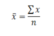
The arithmetic mean is the most common measure of central tendency. The formula of the mean is:

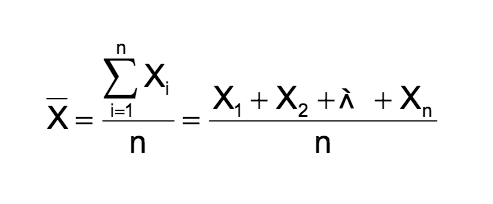
where n stands for the sample size and xn stands for the observed values. This formula is usually written in a slightly different manner using the Greek letter Σ, pronounced “sigma,” which means “sum of.”

The calculation of the Mean in R

In this example, we added the values of 2, 2.5, 3.1, 3.5, 4.3, 4.5, 5 but you can add any values you desire.
>x <- c(2,2.5,3.1,3.5,4.3,4.5,5)
>mean(x)
[1] 3.557143

The Median

The median is the middle score for a set of data that has been arranged in order of magnitude; in other words, 50% of the observations are smaller and 50% of the observations are larger.

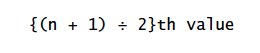
This formula corresponds to these two rules:
Rule 1: If there is an odd number of observations in the dataset, the median is represented by the numerical value corresponding to the positioning point of the ordered observations.

Rule 2: If there is an even number of observations in the dataset, then the positioning point lies between the two observations in the middle of the dataset.

The calculation of the Median in R

In this example, we use the same values 2, 2.5, 3.1, 3.5, 4.3, 4.5, 5 but you can add any values you desire.
>x <- c(2,2.5,3.1,3.5,4.3,4.5,5)
>median (x)
[1] 3.5

The Mode

The mode is the value that occurs most often in the dataset. Unlike  the mean, the mode is not affected by the occurrence of any extreme values. In same cases, we will encounter that we do not have mode. In our example, we do not have mode.

The calculation of the Mode in R

>x <c(2,2.5,3.1,3.5,4.3,4.5,5)
>mode(x)
>”numeric”
The term “numeric” means that R did not find any mode in this dataset.

The Variance

The variance of your data is a measure of spread that will take into account both the deviations of your data (away from the mean) and how frequently these deviations occur. For each data point, the mean is subtracted from the data point, and this value is squared. These squared values are added together and divided by either n or n – 1. If you sampled an entire population, then you divide by n. If you sampled a subset of a population, you divide by n-1. The formula for calculating variance is:

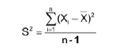
X¯ = Mean
n = sample size
X1 = ith value of variable x

The calculation of the Variance in R

>x <c(2,2.5,3.1,3.5,4.3,4.5,5)
>var (x)
[1] 1.212857

The result, in our dataset, is that the variance is equal to 1.212857.

The Standard Deviation

The most practical and most commonly used measure of variation is the standard deviation, which is represented by the symbol S. It shows how much variation, or dispersion, there is from the average (mean, or expected/budgeted value). A low standard deviation indicates that the data points tend to be very close to the mean, whereas high standard deviation indicates that the data is spread out over a large range of values.

Where x represents each value in the population, x is the mean value of the sample, Σ is the summation (or total), and n-1 is the number of values in the sample minus 1.

The calculation of the Standard Deviation in R

>x <c(2,2.5,3.1,3.5,4.3,4.5,5)
>sd (x)
[1] 1.101298

The result is that the value of standard deviation is equal to 1.101298

 

Next, Chapter 6 Bivariate Statistics
Previous, Chapter 4, How to Run R?